Policy Gradient Toolbox: Overview and Implemented Functions

When I got started with policy gradient reinforcement learning, there were few possibilities how I could have simply tried out existing methods on well-understood problems in order to understand the underlying problems of policy gradient methods. Using this toolbox, I developed a variety of interesting algorithms which I hereby share with the scientific community.

I am currently working on a journal paper covering this area, and I am attempting to put every example which I create as a matlab file on this website so that readers and reviewers can verify my results. Please my website and publciations for further results.

In the remainder of this page, we give an overview on the different constructs which are being offered by the policy gradient toolbox. We divided them up among the following categories.

Problem specific constructs allow you to define your system.
Policy specific constructs allow you to define your policy.
Foundations constructs allow you determine all kind of distributions of states, etc., value functions, the expected return, and the optimal policy for that particular problem.
Analytically determined policy gradients are practical for comparing policy gradient estimators in terms of efficiency, and biasedness.
Functions for collecting and visualizing data can be important during debugging and learning.
The most important estimators for 'vanilla' policy gradient estimators are given, ...
... as well as the ones for the natural policy gradients.

Reports on how you are going to use these functions as well as references to our work are highly appreciated. If you intend to contact me, feel free to use the email-address above.

Problem Specific Constructs

The problem specific functions and parameters allow you to define your problem. We consider two kind of problems, discrete problems and linear-quadratic regulation problems as these are well-studied in the literature. The resulting constructs are given in the table below.

Construct	Discrete Problems	LQR Problems
Choose problem type	`initializeDiscreteProblem;`	`initializeLQRProblem;`
Problem size or dimensionality	Number of states `N` Number of actions `M`	State dimensionality `N`
Discount factor γ	Average reward `gamma = 1;` Discounted reward, e.g., `gamma = 0.95;`	Average reward `gamma = 1;` Discounted reward, e.g., `gamma = 0.95;`
Start-state probability	Start state probability table`p0(x).`	Gaussian start-state distribution with mean `my0` and covariance `S0`. Beware of making `S0` too small - the discounted distribution becomes an infinite peak in that case.
Draw the start-state	`x0=drawStartState;`	`x0=drawStartState;`
State transition parameters	Transition table `p(x,u,xn)`	Transition matrix `A` and coupling vector `b`
Draw next state xnext given current state x and current action u.	`xnext=drawNextState(x,u)`	`xnext=drawNextState(x,u)`
Reward parameters	Reward table `r(x,u)`	State reward matrix `Q` and action reward matrix `R`.
Obtain reward	`rew=rewardFnc(x,u);`	`rew=rewardFnc(x,u);`

These are all problem specific constructs which are not influenced by the policy at all. The constructs for defining the policy are given on the next page

Policy Specific Constructs

In the policy gradient library, we have implemented three types of policies, i.e., the decision border policy, the ε-soft Gibbs policy, and the Gaussian policy. The following constructs are policy specific and given for them.

Construct	Matlab Function
Initialize policy π_θ_'.	Decision border policy: `policy = initDecisionBorderPolicy;` ε-soft Gibbs policy: `epsilon = 1;` `policy = initEpsSoftGibbsPolicy(epsilon);` Gaussian policy: `policy = initGaussPolicy;`
Policy parameters θ	Decision border policy (N*(M-1) parameters): `policy.theta` ε-soft Gibbs policy (NM parameters): `policy.theta` Gaussian policy parametersθ = [k, θ]^T: `policy.theta.k` `policy.theta.sigma`
Probability of taking action u in state x.	`probability = pi_theta(policy, x,u)`
Draw an action from the policy π_θ	`u = drawAction(policy, x);`
Calculate the derivative of the logarithm of the policy log π_θ with respect to the parameters θ.	`derivative = DlogPiDTheta(policy, x, u);`

These are all policy specific functions; all policies have to be initialized with build in functions - otherwise an unproblematic usage of the library cannot be guaranteed.

Foundations Constructs

In this section, we will review all constructs which we need to obtain policy gradients, i.e., the foundations of the policy gradients: stationary and discounted distribution, expected rewards, value and advantage functions.

Construct	MATLAB Function
Stationary distribution d^π(x)	`probability = stationaryDistribution(policy, x)`
Discounted distribution d^π_θ(x)	`probability = discountedDistribution(policy, x)`
State value function V^π(x)	`value = VFnc(policy, x)`
State-action function Q^π(x,u)	`value = QFnc(policy, x, u)`
Advantage function A^π(x,u)	`advantage = AFnc(policy, x, u)`
Expected reward J(π_θ)	`value = expectedReward(policy)`
Optimal policy π_θ^*	`optimalPolicy = optimalSolution(policy)`

Additional to these functions, we have implemented the transition kernels; however, as these become difficult to handle, we do not support them on this webpage. The code is included in the library - feel free to experiment.

Analytically Determined Policy Gradients

There are two types of gradients implemented, i.e., the policy gradient and the natural policy gradient. The latter one also gives the parameters of the compatible function approximation. The policy gradient can be constructed out of the all-action or Fisher information matrix by dJdtheta = M * w.

Construct	MATLAB Code
Policy gradient dJ(π_θ)/dθ	`dJdtheta = policyGradient(policy)`
Natural policy gradient or compatible function approximation parameters w_θ	`w = naturalPolicyGradient(policy)`
Calculate the all-action or Fisher information matrix.	`M = allActionMatrix(policy)`

We will be happy to add more complicated gradients such as the Hessians if you can derive them in a closed form.

Collect and Visualize Data

Policy gradient methods are not about obtaining results analytically but about algorithms which compute these results from empirically obtained data. However, checking the data is often the key to success.

Data is collected in form of trajectories and specified in the format:

% Data specification

: % States in trajectory i in the order as visited
: data.traj(i).x = [x0 x1 x2...xn];
: % Actions in trajectory i in the order as executed
: data.traj(i).u = [u0 u1 u2...un];
: % Rewards in trajectory i in the order as received
: data.traj(i).r = [r0 r1 r2 r3...rn];

In here, there has to be at least one trajectory and all trajectories have to be numbered consecutively. When this is achieved, you can visualize the state distributions using the following commands.

Construct	MATLAB Code
Obtain a single trajectory (number h) of length L	`data(h) = obtainData(policy, L)`
Obtain H trajectories of length L	`data = obtainData(policy, L, H)`
Show the distribution of the states in the given data (using color1) together with the analytical stationary distribution (using color2).	`showStateDistribution(data, policy, color1, color2)`
Show the discounted distribution of the states in the given data (using color1) together with the analytical discounted distribution (using color2).	`showDiscountedStateDistribution(data, policy, color1, color2)`
Show the empirical value function together with the analytical one;	`showEmpiricalValueFunction(data);`

In case you want to add another function, just email us.

'Vanilla' Policy Gradient Estimators

In the table below, we list the most importantpolicy gradient algorithms, i.e., REINFORCE, episodic REINFORCE, and GPOMDP. Please note that (nonepisodic) REINFORCE is in fact a biased policy gradient estimator. In any case, try out the following gradient estimators on your sample problem:

Policy Gradient Estimator	MATLAB Code
Non-episodic REINFORCE	`dJdtheta = nonepisodicREINFORCE(policy, data)`
Episodic REINFORCE	`dJdtheta = episodicREINFORCE(policy, data)`
GPOMDP	`dJdtheta = GPOMDP(policy, data)`

In case you want to add another algorithm, just email us.

Natural Policy Gradient Estimators

In here, the three basic approaches of obtaining the natural policy gradient are presented. The direct direct approximation (i.e., projecting the state-action value function onto the advantage function) suggested by Konda et al. and Sutton et al., the seperate estimation of a state-value function and the subsequent estimation of the gradient, SARSA (which is a biased approximation of the natural policy gradient), natural actor-critic (with good additional basis functions), and episodic natural actor-critic (with no additional basis functions). Their usage is described below.

Natural Policy Gradient Est.	MATLAB Code
Direct Approximation	`w = directApproximation(policy, data)`
Seperate estimation of a state-value function and the subsequent estimation of the gradient	`w = learnThroughValueFunction(policy, data)`
Natural Actor-Critic	`w = naturalActorCritic(policy, data)`
EpisodicNaturalActorCritic	`w = episodicNaturalActorCritic(policy, data)`

In case you want to add another algorithm, just email us.

Example I: Discrete Problems

Discrete problems have been the most traditional example in reinforcement learning. The most likely reason for this is that the many computer scientists apply reinforcement learning methods - and CS problems are usually discrete.
For this page, we have implemented a short library of MATLAB scripts for discrete problems. This library gives you the opportunity to generate examples and test out policy gradient algorithms. On this page, we will shortly show how you can encode a problem using the Two-State Problem presented in the paper; it can be seen in Figure 1.

Figure 1: This figure shows the basic two state problem with two actions

We will proceed as follows: first, we will show you how to encode a discrete problem if you have the transition probabilities, and (expected) rewards for all actions and states. Second, we will show how you select an initial policy. Third, we will show how you can obtain the foundations of policy gradients: transition and resolvent kernels, stationary and discounted distributions, expected returns, value and advantage functions. Fourth, we will show you how you can obtain the main ingredients for policy gradient methods, i.e., the policy gradient, and the natural policy gradient. Finally, you can download the whole package...

Encoding the Problem

In order to use the library, you have to encode the problem. First, you have to declare the global variables and select the problem type.

: % Declare global variables
: global N M p r gamma
: initDiscreteProblem;

Then you have select the problem size, i.e., set the number of states N and actions M.

: % Set problem size
: N = 2; % Set number of states
: M = 2; % Set number of actions

transition probabilities. The transition probability table of the Two State problem is given in Table 1.

Table 1: This figure shows the transition probability table of the two state problem with

two actions. As the problem is deterministic, all table entries are zeros and ones.

Below, you can see how you can encode a transition from one state to the next state given an action, this is done in the form p(x,u,x').

: % Transition table p(x, u, x') -> [0, 1]
: p(1,1,1) = 1; p(1,2,1) = 0;
: p(1,2,2) = 1; p(1,1,2) = 0;
: p(2,1,1) = 1; p(2,2,1) = 0;
: p(2,2,2) = 1; p(2,1,2) = 0;

The rewards are usually also given in tabular form. Table 2 shows the rewards of the two state problem.

Table 2: This figure shows the (expected) reward table of the two state problem

with two actions.

The library requires you to specify all rewards as shown below. The format is r(x,u).

: % Reward table r(x, u) -> IR
: r(1,1) = 2; r(1,2) = 0;
: r(2,1) = 0; r(2,2) = 1;

Furthermore, you have to select the type of problem. You can select it to be either an average reward or a discounted problem. For the average reward formulation, you select the following.

: % Average reward formulation
: gamma = 1;

For the discounted formulation, you have to set the variable gamma to the value of the discount factor γ. E.g., if this discount factor ? has the value 0.95, we have

: % Discounted reward formulation
: gamma = 0.95;

This is a complete specification of the environment and problem. However, we still have to specify the policy.

Encoding the Policy

In discrete problems, we first have to decide which policy is appropriate for our problem: a Gibbs policy or a decision border policy. In this library, we have implemented only the ε-soft Gibbs policy and not any general Gibbs policy.

: % Select epsilon-soft Gibbs policy with epsilon = 1
: epsilon = 1;
: policy = initEpsSoftGibbsPolicy(epsilon);

Furthermore, we have implemented the decision border policy. This can be initialized by

: % Select a decision border policy
: policy = initDecisionBorderPolicy;

You can access the policy parameters using the policy variable. For example, if you would want to change the policy parameters of a decision border policy, you can do this by

: % Select initial policy
: policy.theta = [0.43 0.67];

After doing these initializations, we can proceed to the tools provided by this MATLAB library.

Using the Foundations

After encoding both the problem and the policy, you can start applying the library. Let us assume, you intend to plot the stationary distribution and the discounted distribution of the Markov process. In this case, you can obtain it using the following code.

: % Get state distributions...
: for x=1:N
: : : dstat(x) = stationaryDistribution(policy, x);
: : : ddisc(x) = discountedDistribution(policy, x);
: end;

Furthermore, you could plot either of the distributions using the bar(dstat) or bar(ddisc) commands. The output can look like in Figure 2.

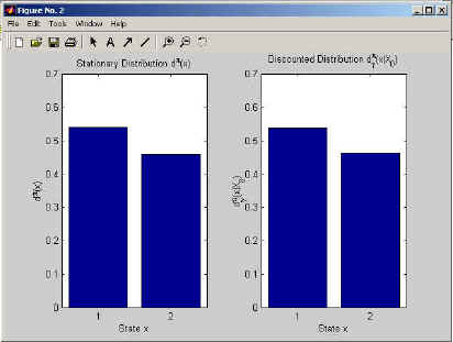
Figure 2: This figure shows the MATLAB output of the stationary and discounted distribution.

Using the function transitionKernel(policy, i, x0, xi) you can obtain the probability of reaching state xi starting from x0 in i steps. Similarly, you can obtain the resolvent kernel, i.e., the discounted probability of reaching state xg starting from x0 discounted by factor γ when using resolventKernel(policy, x0, xg). We will add no further examples on these tools. If you want to try them out use the file KernelsExampleDsc.m.

The next important tool of this library is the expected return. This is obtained using the script expectedReward(policy). This script does not need specifications; it selects the case based on your encoding of the problem and policy. The code below shows a sample program which obtains the expected reward for different policies, so that we can draw a map of the expected reward in parameter space.

: % Calculate the map of expected rewards ...
: for i=0:10
: : : for j=0:10
: : : : : % Set policy parameters
: : : : : policy.theta = [i/10 j/10];
: : : : : % Obtain expected re
: : : : : J_pi(j+1, i+1) = expectedReward(policy);
: : : end;
: end;

In case you want to plot the map of the expected reward in parameter space, we recommend using the function contourf(J_pi) with colormap hot. This gives us Figure 3.

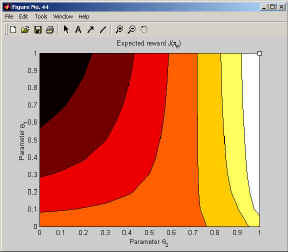
Figure 3: This figure shows the MATLAB output of the map of the expected returns in policy parameter space. The optimal policy is indicated in the upper right corner.

Furthermore, we usually intend to find the optimal solution; for discrete problems, this solution can be determined using the script optimalSolution(policy). The policy in parentheses is only required to determine what kind of policy should be returned by it. You can use it like

% Determine optimal policy: optimalPolicy = optimalSolution(policy);

It is shown as the tiny rectangle in the upper right corner of Figure 3 using plot(optimalPolicy.theta(1), optimalPolicy.theta(2), 'ks').

The last important functions are the value functions. These can be obtained in a similar fashion using the scripts VFnc, QFnc and AFnc. You can obtain the value functions for example using the following code

: % Calculate Value Functions
: for x=1:N
: : : V(x) = VFnc(policy, x);
: : : for u=1:M
: : : : : Q(x,u) = QFnc(policy, x, u);
: : : : : A(x,u) = AFnc(policy, x, u);
: : : end;
: end;

If you want to plot the value, you can do this using bar(V) for the state-value function, and imagesc for the state-action-value function and advantage function; for the later two you can also use our script ShowFunc. An example output is given in Figure 4.

Figure 4: This figure shows the MATLAB output of the value functions.

We now conclude the discussion by saying that the value functions look more impressive for larger problems.

Obtaining Policy Gradients and Natural Policy Gradients

The main functions of the policy gradient library are the policy gradient policyGradient(policy) and the natural policy gradient naturalPolicy Gradient(policy). Using these functions, you can obtain the parameter update of the policy. If you intend to draw a policy gradient map, you can do this using the previously obtained map of the expected return, and the arrow(location,vector,color) function. The following code segment draws a map of the policy gradients and natural policy gradients.

: n_arrows = 15; l_arrows = 1/n_arrows;
: for i=0:n_arrows
: : : for j=0:n_arrows
: : : : : % Set admissable policy parameters
: : : : : policy.theta = [i/n_arrows j/n_arrows];
: : : : : % Calculate Policy Gradient
: : : : : dJdtheta = policyGradient(policy);
: : : : : % Show Policy Gradient
: : : : : subplot(1,2,1);
: : : : : arrow(policy.theta, l_arrows*...
: : : : : dJdtheta/sqrt(sum(dJdtheta.^2)), 'r');
: : : : : % Calculate Natural Gradient
: : : : : w = naturalPolicyGradient(policy);
: : : : : % Show Policy Gradient
: : : : : subplot(1,2,2);
: : : : : arrow(policy.theta, l_arrows*w/sqrt(sum(w.^2)), 'r');
: : : end;
: end;

This program plots the gradient map; it is shown in Figure 5. Additionally to the gradients, the expected reward landscape is being drawn.

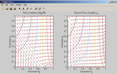
Figure 5: This figure shows the MATLAB output of the map of policy gradients and natural policy gradients.

Figure 5 is worth studying in-depth; we recommend that you try out the whole sample program just due to that one.

Learning the Optimal Policy

To simulate an learning episode, you can use the policy gradient policyGradient(policy) and the natural policy gradient naturalPolicy Gradient(policy). Such a simulation could be done as follows:

: % Set initial policy parameters
: policy.theta = [0.1 0.9];
: % Simulate learning process for policy1 with the policy gradient
: while(isempty(find(policy1.theta<=0 | policy2.theta>=1)))
: : : % Calculate Policy Gradient
: : : dJdtheta = policyGradient(policy1);
: : : % Show desired update
: : : arrow(policy1.theta, 0.1*dJdtheta, 'b');
: : : %Update policy
: : : policy1.theta = policy1.theta + 0.1*dJdtheta;
: end;

By replacing the natural gradient with the policy gradient, we can do the same for that. In Figure 6, we show how four different learning trials look like. These are given in the sample programs; note that the policy gradient rarely reaches the optimal solution - the natural gradient on the other hand reaches it every time.

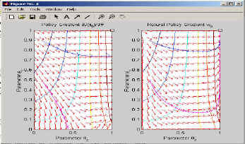
Figure 6: This figure shows the MATLAB output of the map of policy gradients and natural policy gradients with the trials inserted in it.

However, in this section, we have so far obtained every component analytically. Therefore, we will now proceed to trials.

Sample Program

We have made the whole library downloadable. In particular, it includes TwoStateDF.m. This sample program implements all of the given examples for the discounted formulation where the discount factor γ has the value 0.95. A decision border policy is used as it can be plotted for this example. The program is included in the downloadable library.

Example II: Linear Quadratic Regulation

Among non-discrete problems, linear quadratic regulation problems have been the most prominent application of reinforcement learning techniques. Similar to discrete problems, we have included them into the policy gradient library. Again, we have implemented them as MATLAB scripts. The library gives you the opportunity to generate examples and test out policy gradient algorithms. On this page, we will shortly show how you can encode a problem using the one-dimensional linear quadratic regulation problem presented in the paper; it can be seen in Figure 1.

Figure 1: This figure shows a basic one-dimensional linear control problem. In (a), the physical description is given; in (b), the corresponding block diagram is given.

We will proceed exactly like for Case-Study I. If you have read that one carefully, it will be straightforward to understand this case-study.

Encoding the Problem

In order to use the library, you have to encode the problem. First, you have to declare the global variables and initialize the problem type.

: % Declare global variables
: global N A b Q R gamma
: initLQRProblem;

Then you have select the problem dimensionality, i.e., set the dimensionality of the states N.

: % Set problem size
: N = 2; % Set the dimensionality of the states

The initial or start state distribution is in general assumed to be a Gaussian distribution; you can use this distribution t create more difficult ones. For example, when you use a variance close to zero, you get a single start-state distribution. The initial or start state distribution is specified as follows.

: % Start state distribution
: my0 = 0.3*ones(N,1);
: S0 = 0.00001*eye(N);

You have to specify the matrix A, and vector b describing the state transitions, i.e., the state transition equation has to be given in form x_t+1 = Ax_t + bu_t. For our simple these are just scalars; if we set N to a higher value, we obtain matrices.

: % Transition matrix A and vector b
: A = eye(N);
: b = ones(N,1);

The rewards are given as a quadratic form with r(x, u) = x^TQx + u^TRu. The matrix Q and the scalar R have to specified.

: % Reward matrix Q and scalar R
: Q = eye(N);
: R = 1;

Furthermore, you have to select the type of problem. You can select it to be either an average reward or a discounted problem. For the average reward formulation, you select the following.

: % Average reward formulation
: gamma = 1;

For the discounted formulation, you have to set the variable gamma to the value of the discount factor g. E.g., if this discount factor g has the value 0.95, we have

: % Discounted reward formulation
: gamma = 0.95;

This is a complete specification of the environment and problem. However, we still have to specify the policy.

Encoding the Policy

For linear quadratic regulation problems, the library gives us a single choice, i.e., a Gaussian policy. It can be initialized by

: % Select a Gauss policy
: policy = initGaussPolicy;

You can access the policy parameters using the policy variable. For example, if you would want to change the policy parameters of a decision border policy, you can do this by

: % Select initial policy
: policy.theta.k = -1; % Set controller gains...
: policy.theta.sigma = 1; % Set controller variance...

After doing these initializations, we can proceed to the tools provided by this MATLAB library.

Using the Foundations

: % Get state distributions...
: for index=1:80
: : : x(index) = 0.5*(index - 41) / 40;
: : : dstat(index) = stationaryDistribution(policy, ...
: : : : : x(index));
: : : ddisc(index) = discountedDistribution(policy, ...
: : : : : x(index));
: end;

The index is necessary as the addressing number have to be integers. Furthermore, you could plot either of the distributions using the plot(x, dstat) or plot(x, ddisc) commands. The output can look like in Figure 2.

Figure 2: This figure shows the MATLAB output of the stationary and discounted distribution.

Functions like transitionKernel or resolventKernel were not implemented. The reason for this is that the 0-step transition kernel and therefore also the resolvent kernel are infinite for x₀= x.

: % Calculate the map of expected rewards ...
: for i=0:10
: : : % Set controller gain
: : : policy.theta.k = 2*(10-i)/10;
: : : for j=0:10
: : : : : % Set controller variance
: : : : : policy.theta.sigma = j/10;
: : : : : % Obtain expected reward
: : : : : J_pi(j+1, i+1) = expectedReward(policy);
: : : end;
: end;

In case you want to plot the map of the expected reward in parameter space, we recommend using the function contourf(J_pi) with colormap hot. This gives us Figure 3.

Figure 3: This figure shows the MATLAB output of the map of the expected returns in policy parameter space. The optimal policy is indicated with the rectangle.

: % Determine optimal policy
: optimalPolicy = optimalSolution(policy);

It is shown as the tiny rectangle in the upper right corner of Figure 3 using plot(optimalPolicy.theta.k, optimalPolicy.theta.sigma, 'ks').

: % Calculate Value Functions
: for indexX=1:81
: : : x(indexX) = -5+10*(indexX-1) / 80;
: : : VT(indexX) = VFnc(policy, x(indexX));
: : : for indexU=1:81
: : : : : u(indexU)=-5+10*(indexU-1)/80;
: : : : : QT(indexX,indexU)=QFnc(policy, x(indexX),u(indexU));
: : : : : AT(indexX,indexU)=AFnc(policy, x(indexX),u(indexU));
: : : end;
: end;

If you want to plot the value, you can do this using plot(V) for the state-value function, and surf(Q) or contourf(Q)for the state-action-value function and advantage function. An example output is given in Figure 4.

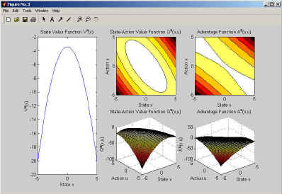
Figure 4: This figure shows the MATLAB output of the value functions.

We now conclude the discussion by saying that the the advantage function looks fairly different to the state-action value function.

Obtaining Policy Gradients and Natural Policy Gradients

: n_arrows = 10; l_arrows = 1/n_arrows;
: for i=0:n_arrows
: : : % Set controller gain
: : : policy.theta.k = 2*(n_arrows-i)/n_arrows;
: : : for j=0:n_arrows
: : : : : % Set controller variance
: : : : : policy.theta.sigma = j/n_arrows;
: : : : : % Calculate Policy Gradient
: : : : : dJdtheta = policyGradient(policy);
: : : : : % Show Policy Gradient
: : : : : subplot(1,2,1);
: : : : : arrow(policy.theta, l_arrows*...
: : : : : dJdtheta/sqrt(sum(dJdtheta.^2)), 'r');
: : : : : % Calculate Natural Gradient
: : : : : w = naturalPolicyGradient(policy);
: : : : : % Show Policy Gradient
: : : : : subplot(1,2,2);
: : : : : arrow(policy.theta,l_arrows*w/sqrt(sum(w.^2)),'r');
: : : end;
: end;

This program plots the gradient map; it is shown in Figure 5. Additionally to the gradients, the expected reward landscape is being drawn.

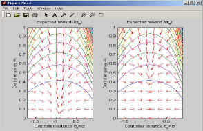
Figure 5: This figure shows the MATLAB output of the map of policy gradients and natural policy gradients.

Figure 5 is worth studying in-depth; we recommend that you try out the whole sample program just due to that one.

Learning the Optimal Policy

To simulate an learning episode, you can use the policy gradient policyGradient(policy) and the natural policy gradient naturalPolicy Gradient(policy). Such a simulation could be done as follows:

: % Select initial policy
: policy.theta.k = -0.1; % Set controller gains...
: policy.theta.sigma = 0.9; % Set controller variance...
: % Simulate learning process for policy1 with the policy
: % gradient
: while(policy1.theta.sigma>=0.1)
: : : % Calculate Policy Gradient
: : : dJdtheta = policyGradient(policy1);
: : : % Show desired update
: : : arrow([policy1.theta.k policy1.theta.sigma], ...
: : : : : 0.025*dJdtheta, 'b');
: : : %Update policy
: : : policy1.theta.k = policy1.theta.k + ...
: : : : : 0.025*dJdtheta(1:N);
: : : policy1.theta.sigma = policy1.theta.sigma + ...
: : : : : 0.025*dJdtheta(N+1);
: end;

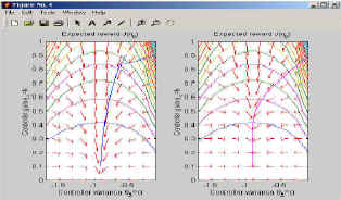
Figure 6: This figure shows the MATLAB output of the map of policy gradients and natural policy gradients with the trials inserted in it.

Sample Program

We have made the whole library downloadable. In particular, it includes LQR1dDF.m. This sample program implements all of the given examples for the discounted formulation where the discount factor γ has the value 0.95. A gaussian policy is used as it can be plotted for this example. The program is included in the downloadable library.

Estimators

Having derived all analytical constructs for the two case studies, we are now interested in how the different estimators of policy and natural policy gradients perform. Policy gradient estimators such as William's non-episodic REINFORCE, William's episodic REINFORCE, Baxter & Bartlett's GPOMDP, Sutton's SARSA (for Gibbs policies) and Suttons, Andersons & Bartos Actor-Critic Architecture have been implemented.

In order to make your usage of these methods as easy as possible, we have parted the data collection from the gradient estimation. This allows you to obtain or specify data - and use exactly the same data for all algorithms. Furthermore, you can not only obtain the gradient estimates but also plot the data and compare it to the analytical constructs.

Collecting Data

First, we have to obtain the data based on our problem specification. To do this, we collect data in form of trajectories and specify them in the format:

: % Data specification
: % States in trajectory in the order as visited
: data(1).x = [x0 x1 x2...xn];
: % Actions in trajectory in the order as executed
: data(1).u = [u0 u1 u2...un];
: % Rewards in trajectory in the order as received
: data(1).r = [r0 r1 r2 r3...rn];

If you want to draw data by yourself, you can do that in the following way: you perform H episodes. An episode consists out of drawing a start-state and subsequently drawing the triple (u_t,r_t,x_t+1) for all steps until the Episode length L is reached.

: % Perform H episodes
: for trials=1:H
: : : % Draw the first state
: : : data(trials).x(1) = drawStartState;
: : : % Perform a trial of length L
: : : for steps=1:L
: : : : : % Draw an action from the policy
: : : : : data(trials).u(steps) = drawAction(policy, ...
: : : : : data(trials).x(steps));
: : : : : % Obtain the reward from the
: : : : : data(trials).r(steps) = rewardFnc(...
: : : : : data(trials).x(steps), data(trials).u(steps));
: : : : : % Draw next state from environment
: : : : : data(trials).x(steps+1) = drawNextState(...
: : : : : data(trials).x(steps), data(trials).u(steps));
: : : end;
: end;

In case that you do not intend to write all that code - don't worry, we have just the functions for you. With the function

: data(h) = obtainTrajectory(policy, L)

you can obtain a single trajectory/episode of length L, and with the function

: data = obtainData(policy, H, L)

you can get the H episodes of length L.

For example, the following code shows you how you can obtain a two trajectories of length 10. Subsequently it asks MATLAB for the values of the trajectories:

: > data = obtainData(policy, 10, 2)
: data = 1x2 struct array with fields:
: policy \\ x \\ u \\ r \\ \\ � data(1).x
: ans = 0.2883 0.2553 0.1612 0.1176 -0.0926 -0.0715 -0.0633 0.0840 0.3053 0.1477 -0.0324

: > data(1).u
: ans = -0.0330 -0.0941 -0.0436 -0.2102 0.0211 0.0082 0.1473 0.2213 -0.1575 -0.1802

: > data(1).r
: ans = -0.0416 -0.0330 -0.0131 -0.0091 -0.0043 -0.0026 -0.0031 -0.0060 -0.0478 -0.0125

Using data(2), you can access the second trajectory. If you leave away the number of trajectories, you always get a single trajectory.

Visualize Data

Obviously, showing all trajectories would be a waste of time as stochastic policies barely exhibit patterns which we can directly detect. However, you can still analyze it well based on histograms of the finite data.

The function

: showStateDistribution(data)

shows a comparison of the obtained data with the stationary distribution. This function works for arbitrary discrete problems; however, for LQR it requires a dimensionality of 1 or 2. Similarly, you can show the empirical discounted distribution in comparison to the analytical one

: showDiscountedStateDistribution(data)

in comparison to the analytical one. The example program VisDataDisc.m visualizes the data of the discrete Two-State-Problem; it is shown in Figure 1. Example program VisDataLQR1d.m visualizes the data of the one dimensional LQR-Problem (see Figure 2) and VisDataLQR2d.m shows the two-dimensional case (see Figures 3 and 4).

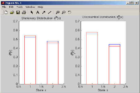
Figure 2: This figure shows the stationary and discounted distributions of a Two-State problem. The bars describe the actual data while the red lines describe analytical distributions to which the bars converge if sufficiently much data is being used.

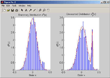
Figure 2: This figure shows the stationary and discounted distributions of a one-dimensional linear control problem. The bars describe the actual data while the red lines describe analytical distributions to which the bars converge if sufficiently much data is being used.

If you intend to provide us with further visualizations - we would love to add them to the library.

Vanilla Policy Gradient Estimators

This function gives us several policy gradient algorithms, i.e., REINFORCE, episodic REINFORCE and GPOMDP. If you want to compare these methods, try

: dJdtheta = nonepisodicREINFORCE(policy, data)
: dJdtheta = episodicREINFORCE(policy, data)
: dJdtheta = GPOMDP(policy, data)

However, you should beware to make judgments without consulting our paper as some of these algorithms just address special cases; e.g., non-episodic REINFORCE does not address the temporal credit assignment problem.

Natural Policy Gradient Estimators

In here, the three basic approaches of obtaining the natural policy gradient are presented: (1) direct approximation (i.e., projecting the state-action value function onto the advantage function as suggested by Kakade or Konda), (2) temporal difference learning (i.e., with additional basis functions) such as naturalActorCritic and learnThroughValueFunction, and (3) sample path based learning such as episodicNaturalActorCritic. These methods are described in the paper. You can obtain the natural gradient with them using the following code.

: w = directApproximation(policy, data)
: w = naturalActorCritic(policy, data)
: w = learnThroughValueFunction(policy, data)
: w = episodicNaturalActorCritic(policy, data)

Finding better methods than these is THE essential problem in policy gradient methods. This is THE topic which we have to investigate in the future.

Download

Copyright (c) 2002, Computational Motor Control Laboratory. All rights reserved. Redistribution and use in source and binary forms, with or without modification, are permitted provided that the following conditions are met:

Redistributions of source code must retain the above copyright notice, this list of conditions and the following disclaimer.
Redistributions in binary form must reproduce the above copyright notice, this list of conditions and the following disclaimer in the documentation and/or other materials provided with the distribution.
Neither the name of the Computational Motor Control Laboratory nor the names of its contributors may be used to endorse or promote products derived from this software without specific prior written permission.
If used in any scientific publications, the publication has to refer specifically to the work published on this webpage.

This software is provided by us "as is" and any express or implied warrenties, including, but not limited to, the implied warrenties of merchantability and fitness for particular purpose are disclaimed. In no event shall the copyright holders or any contributor be liable for any direct, indirect, incidental, special, exemplary, or consequential damages however caused and on any theory of liability whether in contract, strict liability or tort arising in any way out of the use of this software, even if advised of the possibility of such damage.

DOWNLOAD HERE: I agree and therefore I download this toolbox.